Python TensorFlow: Experimenting with Learning Rates in Gradient Descent

Python TensorFlow Building and Training a Simple Model: Exercise-12 with Solution

Write a Python program to experiment with different learning rates in a gradient descent optimizer and observe the impact on convergence in TensorFlow.

Sample Solution:

Python Code:

import tensorflow as tf
import numpy as np
import matplotlib.pyplot as plt

# Generate some random data for a simple linear regression problem
np.random.seed(0)
X = np.random.rand(100, 1)
y = 2 * X + 1 + 0.1 * np.random.randn(100, 1)

# Define a range of learning rates to experiment with
learning_rates = [0.001, 0.01, 0.1, 0.5]

# Initialize a list to store training histories for each learning rate
training_histories = []

# Train models with different learning rates
for lr in learning_rates:
    # Define the neural network model
    model = tf.keras.Sequential([
        tf.keras.layers.Input(shape=(1,)),
        tf.keras.layers.Dense(1)
    ])
    
    # Define the mean squared error (MSE) loss function
    loss_function = tf.keras.losses.MeanSquaredError()
    
    # Define the gradient descent optimizer with the current learning rate
    optimizer = tf.keras.optimizers.SGD(learning_rate=lr)
    
    # Compile the model with the optimizer and loss function
    model.compile(optimizer=optimizer, loss=loss_function)
    
    # Training loop
    num_epochs = 100
    history = model.fit(X, y, epochs=num_epochs, verbose=0)
    training_histories.append(history.history['loss'])

# Plot the loss curves for different learning rates
plt.figure(figsize=(10, 6))
for i, lr in enumerate(learning_rates):
    plt.plot(range(num_epochs), training_histories[i], label=f'LR={lr}')
plt.xlabel('Epochs')
plt.ylabel('Loss')
plt.legend()
plt.title('Loss Curves for Different Learning Rates')
plt.show()

Output:

Explanation:

Import Libraries:

import tensorflow as tf
import numpy as npimport tensorflow as tf
import numpy as np
import matplotlib.pyplot as plt

Import the necessary libraries: TensorFlow (tf), NumPy (np), and Matplotlib (plt) for data generation and visualization.

-----------------------------------------------------

Generate Random Data:

np.random.seed(0)
X = np.random.rand(100, 1)
y = 2 * X + 1 + 0.1 * np.random.randn(100, 1)

Generate random input data X and target data y for a simple linear regression problem. X is a 2D array with 100 samples and 1 feature, and y is the corresponding target values.

------------------------------------------------------

Define Learning Rates to Experiment With:

learning_rates = [0.001, 0.01, 0.1, 0.5]

We define a list of learning rates to experiment with. You can adjust this list to include different learning rates you want to explore.

---------------------------------------------------------

Initialize a List for Training Histories:

training_histories = []

We create an empty list training_histories to store the training histories (loss curves) for each learning rate.

------------------------------------------------------------

Train Models with Different Learning Rates:

for lr in learning_rates:
    model = tf.keras.Sequential([
        tf.keras.layers.Input(shape=(1,)),
        tf.keras.layers.Dense(1)
    ])
    loss_function = tf.keras.losses.MeanSquaredError()
    optimizer = tf.keras.optimizers.SGD(learning_rate=lr)
    model.compile(optimizer=optimizer, loss=loss_function)
    num_epochs = 100
    history = model.fit(X, y, epochs=num_epochs, verbose=0)
    training_histories.append(history.history['loss'])

• Loop through each learning rate (lr) in the learning_rates list.
• For each learning rate, we define a simple linear regression model with a single input feature and one output unit.
• Specify the mean squared error (MSE) loss function and the gradient descent optimizer with the current learning rate.
• The model is compiled with the optimizer and loss function.
• Train the model for a fixed number of epochs (num_epochs) and store the training loss history in the training_histories list.

------------------------------------------------------------

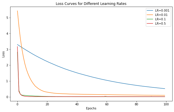
Plot Loss Curves:

plt.figure(figsize=(10, 6))
for i, lr in enumerate(learning_rates):
    plt.plot(range(num_epochs), training_histories[i], label=f'LR={lr}')
plt.xlabel('Epochs')
plt.ylabel('Loss')
plt.legend()
plt.title('Loss Curves for Different Learning Rates')
plt.show()

• Finally, we use Matplotlib to plot the loss curves for different learning rates. Each learning rate's loss curve is displayed on the same plot for comparison.
• The x-axis represents the number of training epochs, and the y-axis represents the loss value.
• The legend shows the learning rates associated with each curve, allowing you to observe how different learning rates affect the convergence behavior of the model.

Python Code Editor:

Previous: Training Neural Networks with Adam Optimizer.