Pandas Series: plot.density() function

Last update on September 15 2022 12:54:43 (UTC/GMT +8 hours)

Series-plot.density() function

In statistics, kernel density estimation (KDE) is a non-parametric way to estimate the probability density function (PDF) of a random variable. This function uses Gaussian kernels and includes automatic bandwidth determination.

The plot.density() function generates Kernel Density Estimate plot using Gaussian kernels.

Syntax:

Series.plot.density(self, bw_method=None, ind=None, **kwargs)

Parameters:

Name	Description	Type/Default Value	Required / Optional
bw_method	The method used to calculate the estimator bandwidth. This can be 'scott', 'silverman', a scalar constant or a callable. If None (default), 'scott' is used. See scipy.stats.gaussian_kde for more information.	str, scalar or callable	Optional
ind	Evaluation points for the estimated PDF. If None (default), 1000 equally spaced points are used. If ind is a NumPy array, the KDE is evaluated at the points passed. If ind is an integer, ind number of equally spaced points are used.	NumPy array or integer	Optional
**kwds	Additional keyword arguments are documented in pandas.%(this-datatype)s.plot().		Optional

Returns: matplotlib.axes.Axes or numpy.ndarray of them.

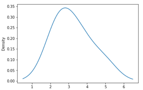
Example - Given a Series of points randomly sampled from an unknown distribution, estimate its PDF using KDE with automatic bandwidth determination and plot the results, evaluating them at 1000 equally spaced points (default):

Python-Pandas Code:

import numpy as np
import pandas as pd
s = pd.Series([2, 3, 2.6, 3.5, 2.5, 4, 5])
ax = s.plot.kde()

Output:

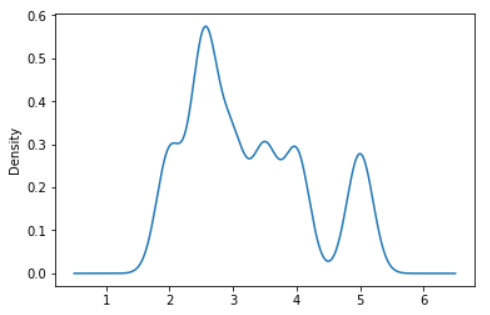
Example - A scalar bandwidth can be specified. Using a small bandwidth value can lead to over-fitting, while using a large bandwidth value may result in under-fitting:

Python-Pandas Code:

import numpy as np
import pandas as pd
s = pd.Series([2, 3, 2.6, 3.5, 2.5, 4, 5])
ax = s.plot.kde(bw_method=0.2)

Output:

Python-Pandas Code:

import numpy as np
import pandas as pd
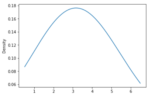
s = pd.Series([2, 3, 2.6, 3.5, 2.5, 4, 5])
ax = s.plot.kde(bw_method=2)

Output:

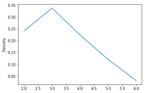
Example - Finally, the ind parameter determines the evaluation points for the plot of the estimated PDF:

Python-Pandas Code:

import numpy as np
import pandas as pd
s = pd.Series([2, 3, 2.6, 3.5, 2.5, 4, 5])
ax = s.plot.kde(ind=[2, 3, 4, 5, 6])

Output:

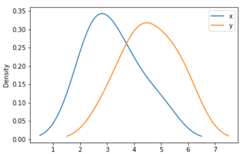
Example - For DataFrame, it works in the same way:

Python-Pandas Code:

import numpy as np
import pandas as pd
df = pd.DataFrame({
    'x': [2, 3, 2.6, 3.5, 2.5, 4, 5],
    'y': [4, 3, 4.5, 4, 5, 5.5, 6],
})
ax = df.plot.kde()

Output:

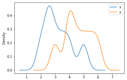
Example - A scalar bandwidth can be specified. Using a small bandwidth value can lead to over-fitting, while using a large bandwidth value may result in under-fitting:

Python-Pandas Code:

import numpy as np
import pandas as pd
df = pd.DataFrame({
    'x': [2, 3, 2.6, 3.5, 2.5, 4, 5],
    'y': [4, 3, 4.5, 4, 5, 5.5, 6],
})
ax = df.plot.kde(bw_method=0.3)

Output:

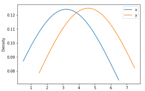
Python-Pandas Code:

import numpy as np
import pandas as pd
df = pd.DataFrame({
    'x': [2, 3, 2.6, 3.5, 2.5, 4, 5],
    'y': [4, 3, 4.5, 4, 5, 5.5, 6],
})
ax = df.plot.kde(bw_method=3)

Output:

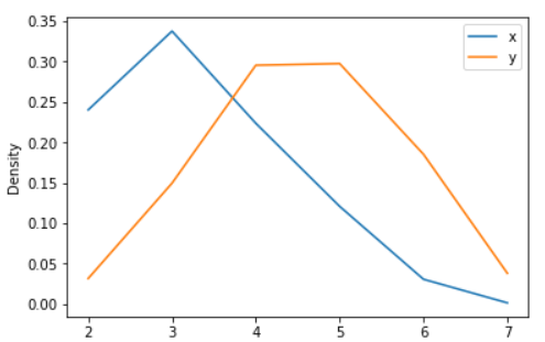
Example - Finally, the ind parameter determines the evaluation points for the plot of the estimated PDF:

Python-Pandas Code:

import numpy as np
import pandas as pd
df = pd.DataFrame({
    'x': [2, 3, 2.6, 3.5, 2.5, 4, 5],
    'y': [4, 3, 4.5, 4, 5, 5.5, 6],
})
ax = df.plot.kde(ind=[2, 3, 4, 5, 6, 7])

Output:

Previous: Series-plot.box() function
Next: Series-plot.hist() function