Excel Formulas - Count rows matching two criterias in two columns within a row

Count rows in a table when they match two criterias in two columns within a row

Syntax of used function(s)

COUNTIFS(criteria_range1, criteria1, [criteria_range2, criteria2]…)

The COUNTIFS function applies criteria to cells across multiple ranges and counts the number of times all criteria are met

Explanation

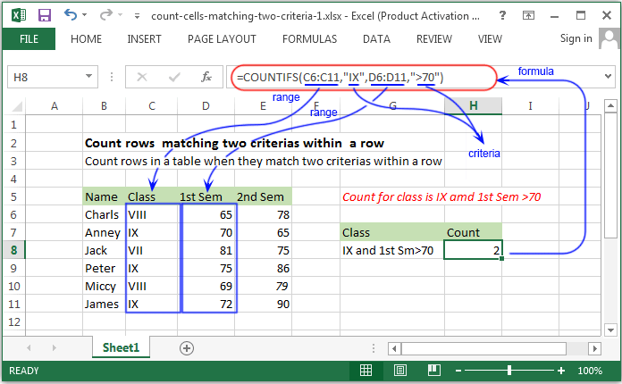
To count the number of rows where two cirterias are matching the COUNTIFS function can be used. In this example we want to count the class is IX and the marks in 1st sem is more than 70.

Formula

=COUNTIFS(C6:C11,"IX",D6:D11,">70")

How this formula works

In the above example the COUNTIFS function accepts multiple criteria in pairs - each pair contains one range and the criteria associated with the range. The count of rows only generated when both the criteria matches.

Count rows matching two criterias in two columns within a row with SUMPROUDCT()

Syntax of used function(s)

SUMPRODUCT(array1, [array2], [array3], ...)

The SUMPRODUCT function is used to multiplies the corresponding components in the given arrays, and returns the sum of those products.

What to do?

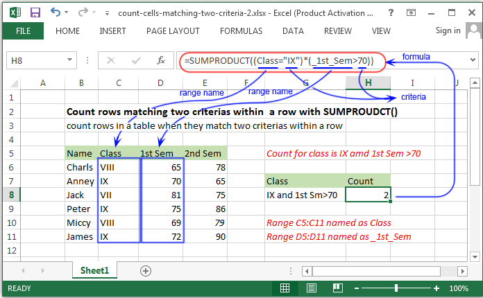
The given table contains the name, class, score of 1st semister and 2nd semister of some students. The count of rows will be generated, when in a same row the class is IX and the score of 1st sem is more than 70.
The uses of SUMPRODUCT function is a good way to solve this problem, because the SUMPRODUCT function can handled the array operations.

Formula

=SUMPRODUCT((Class="IX")*(_1st_Sem>70))

How this formula works

The default behaviour of SUMPRODUCT function is to multiply corresponding elements in one or more arrays together, then sum the products.
In case of given a single array, it returns the sum of the elements in the array.
In the above example, two logical expression have used inside a single argument. After evaluation of two logical expression the formula looks like:

=SUMPRODUCT(({FALSE;TRUE;FALSE;TRUE;FALSE;TRUE;})*({FALSE;FALSE;TRUE;TRUE;FALSE;TRUE;}))

The multiplication operator have been used to multiply the two arrays together and excel will automatically convert the logical value to ones and zeros.
After multiplication, the formula looks like -

=SUMPRODUCT({0;0;0;1;0;1;})

And finally with only one array, SUMPRODUCT simply adds up the elements in the array and returns the sum.

Previous: Excel Formulas - Count number of rows for a specific matching value
Next: Excel Formulas - Count number of rows containing multiple OR condition