Excel Formulas - Count multiple criterias using logical NOT

Count multiple criterias using logical NOT

Syntax of used function(s)

SUMPRODUCT(array1, [array2], [array3], ...)
ISNA(value)
MATCH(lookup_value, lookup_array, [match_type])

The SUMPRODUCT function is used to multiplies the corresponding components in the given arrays, and returns the sum of those products.
The ISNA funtion returns True if the Value refers to the #N/A (value not available) error value.
The MATCH function searches for a specified item in a range of cells, and then returns the relative position of that item in the range.

What to do?

To count with multiple criterias using the logic NOT one of several things, the SUMPRODUCT function together with the MATCH and ISNA functions can be used to solve the problem.

Formula

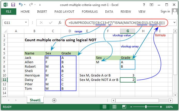
=SUMPRODUCT((C6:C13=F7)*ISNA(MATCH(D6:D13,G7:G8,0)))

How the formula works

In the above example the first expression C6:C13=F7 means that, the SUMPRODUCT function test the value in the range C6:C13 against the value in criteria variable F7, "Male".

The result is an array of TRUE FALSE values like -

 
{TRUE;FALSE;TRUE;FALSE;TRUE;FALSE;TRUE;TRUE;}

The second expression the MATCH function is used to match every value in the range D6:D13 against the values in G7:G8, i.e. "A" and "B". MATCH returns the relative position of that lookup_value in the lookup_arry where match succeeds. It returns a number. Where match failed MATCH returns #N/A.

The results is an array like -

{1;2;1;2;#N/A;#N/A;#N/A;2;}

Since #N/A values correspond to "not A or B", ISNA "reverse" the array to TRUE and FALSE and looks like -

{FALSE;FALSE;FALSE;FALSE;TRUE;TRUE;TRUE;FALSE;}

Now TRUE indicates to "not A or B".

The SUMPRODUCT function now multiplied the two array results, and creates a single numeric array inside SUMPRODUCT and the formula looks like -

=SUMPRODUCT({0;0;0;0;1;0;1;0;})

And finally the SUMPRODUCT produced the sum of the array. Accrodeng to the above example the result is 2.

In the above picture the formula written in G10 is =SUMPRODUCT((C6:C13=F7)*ISNA(MATCH(D6:D13,G7:G8,-1))). In the MATCH function the -1 have been used. That returns an array looks like -

{1;#N/A;1;#N/A;#N/A;#N/A;#N/A;#N/A;}

The ISNA "reverse" the array to TRUE and FALSE and looks like -

{FALSE;TRUE;FALSE;TRUE;TRUE;TRUE;TRUE;TRUE;}

The SUMPRODUCT function now multiplied the two array results, and creates a single numeric array inside SUMPRODUCT and the formula looks like -

=SUMPRODUCT({0;0;0;0;1;0;1;1;})

And finally the SUMPRODUCT produced the sum of the array. Accrodeng to the above example the result is 3.

Previous: Excel Formulas - Count number of cells ends with string
Next: Excel Formulas - Count cells with OR condition